Solving Real World Issues With RCzechia
Jindra Lacko
2024-11-25
Source:vignettes/vignette.Rmd
vignette.RmdVisualizing Czech Population
Population of the Czech Republic from the 2011 census, per district (okres). The results can be easily accessed from the comfort of your R session using the excellent package {czso} by Petr Bouchal.
As the population distributed highly unevenly a log scale is used.
library(RCzechia)
library(ggplot2)
library(readxl)
library(dplyr)
library(httr)

tf <- tempfile(fileext = ".xls") # a temporary xls file
GET("https://raw.githubusercontent.com/jlacko/RCzechia/master/data-raw/zvcr034.xls",
    write_disk(tf))
## Response [https://raw.githubusercontent.com/jlacko/RCzechia/master/data-raw/zvcr034.xls]
##   Date: 2024-11-25 14:10
##   Status: 200
##   Content-Type: application/octet-stream
##   Size: 44.5 kB
## <ON DISK>  /tmp/Rtmpn3okFy/file20e11aee97ca.xls
src <- read_excel(tf, range = "Data!B5:C97") # read in with original column names

colnames(src) <- c("NAZ_LAU1", "obyvatel") # meaningful names instead of the original ones
src <- src %>%
  mutate(obyvatel = as.double(obyvatel)) %>%
    # convert from text to number
  mutate(NAZ_LAU1 = ifelse(NAZ_LAU1 == "Hlavní město Praha", "Praha", NAZ_LAU1))
    # rename Prague (from The Capital to a regular city)

okresni_data <- RCzechia::okresy("low") %>% # data shapefile
  inner_join(src, by = "NAZ_LAU1")
    # key for data connection - note the use of inner (i.e. filtering) join

# report results
ggplot(data = okresni_data) +
  geom_sf(aes(fill = obyvatel), colour = NA) +
  geom_sf(data = RCzechia::republika("low"), color = "gray30", fill = NA) +
  scale_fill_viridis_c(trans = "log", labels = scales::comma) +
  labs(title = "Czech population",
       fill = "population\n(log scale)") +
  theme_bw() +
  theme(legend.text = element_text(hjust = 1),
        legend.title = element_text(hjust = 0.5))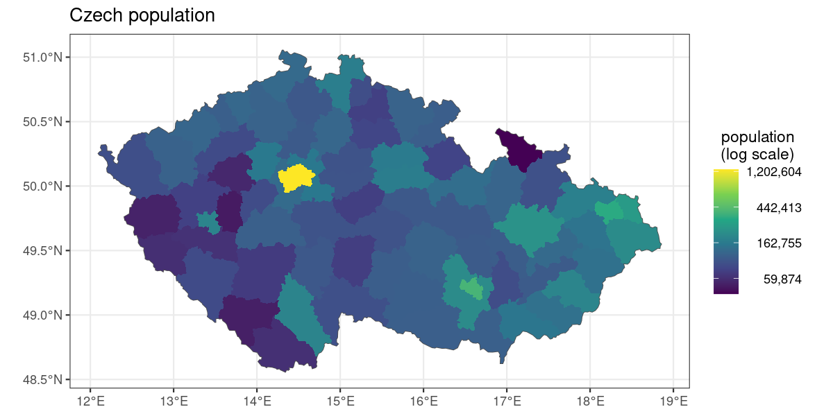
plot of chunk census
Geocoding Locations & Drawing them on a Map
Drawing a map: three semi-random landmarks on map, with rivers shown for better orientation.
To get the geocoded data frame function
RCzechia::geocode() is used.
library(RCzechia)
library(ggplot2)
library(sf)

borders <- RCzechia::republika("low")

rivers <- subset(RCzechia::reky(), Major == T)

mista <- data.frame(misto =  c("Kramářova vila",
                               "Arcibiskupské zahrady v Kroměříži",
                               "Hrad Bečov nad Teplou"),
                    adresa = c("Gogolova 212, Praha 1",
                               "Sněmovní náměstí 1, Kroměříž",
                               "nám. 5. května 1, Bečov nad Teplou"))

# from a string vector to sf spatial points object
POI <- RCzechia::geocode(mista$adresa)

class(POI) # in {sf} package format = spatial and data frame
## [1] "sf"         "data.frame"

# report results
ggplot() +
  geom_sf(data = POI, color = "red", shape = 4, size = 2) +
  geom_sf(data = rivers, color = "steelblue", alpha = 0.5) +
  geom_sf(data = borders, color = "grey30", fill = NA) +
  labs(title = "Very Special Places") +
  theme_bw()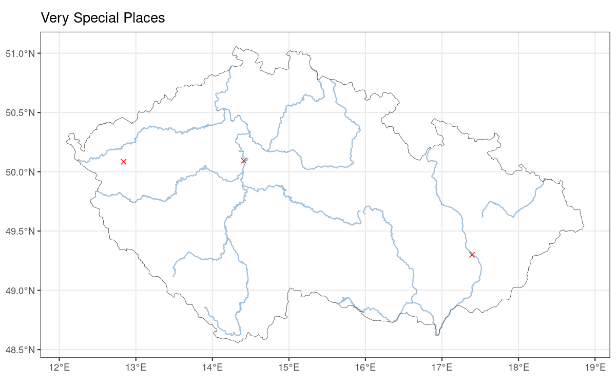
plot of chunk geocode
Distance Between Prague and Brno
Calculate distance between two spatial objects; the sf
package supports (via gdal) point to point, point to polygon and polygon
to polygon distances.
Calculating distance from Prague (#1 Czech city) to Brno (#2 Czech city).
library(dplyr)
library(RCzechia)
library(sf)
library(units)

obce <- RCzechia::obce_polygony()

praha <- subset(obce, NAZ_OBEC == "Praha")

brno <- subset(obce, NAZ_OBEC == "Brno")

vzdalenost <- sf::st_distance(praha, brno) %>%
  units::set_units("kilometers") # easier to interpret than meters, miles or decimal degrees..

# report results
print(vzdalenost[1])
## 152.4642 [kilometers]
Geographical Center of the City of Brno
The metaphysical center of the Brno City is well known. But where is the geographical center?
The center is calculated using sf::st_centroid() and
reversely geocoded via RCzechia::revgeo().
Note the use of reky("Brno") to provide the parts of
Svitava and Svratka relevant to a map of Brno city.
library(dplyr)
library(RCzechia)
library(ggplot2)
library(sf)

# all districts
brno <- RCzechia::okresy() %>%
  dplyr::filter(KOD_LAU1 == "CZ0642")

# calculate centroid
pupek_brna <- brno %>%
  sf::st_transform(5514) %>% # planar CRS (eastings & northings)
  sf::st_centroid(brno) # calculate central point of a polygon

# the revgeo() function takes a sf points data frame and returns it back
# with address data in "revgeocoded" column
adresa_pupku <- RCzechia::revgeo(pupek_brna) %>%
  pull(revgeocoded)

# report results
print(adresa_pupku)
## [1] "Žižkova 513/22, Veveří, 61600 Brno"

ggplot() +
  geom_sf(data = pupek_brna, col = "red", shape = 4) +
  geom_sf(data = reky("Brno"), color = "skyblue3") +
  geom_sf(data = brno, color = "grey50", fill = NA) +
  labs(title = "Geographical Center of Brno") +
  theme_bw()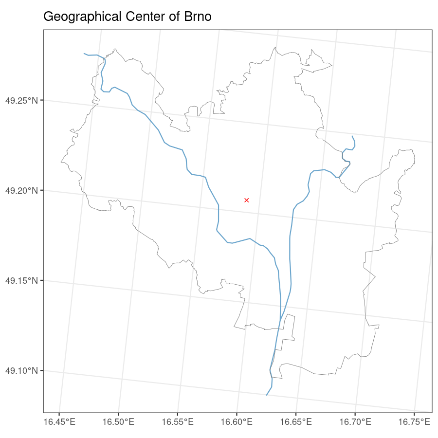
plot of chunk brno-center
Interactive Map
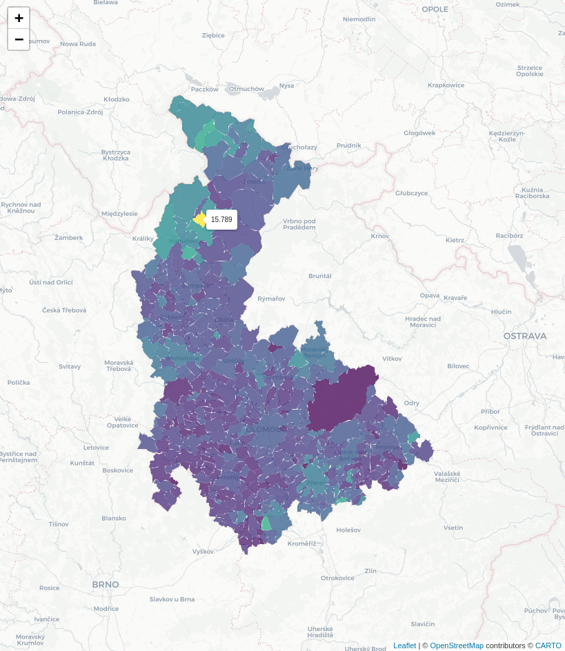
Interactive maps are powerful tools for data visualization. They are
easy to produce with the leaflet package.
Since Stamen Toner basemap no longer sparkles joy I have found a new favorite - the Positron by CartoDB.
Note: it is technically impossible to make html in vignette interactive (and for good reasons). As a consequence the result of code shown has been replaced by a static screenshot; the code itself is legit.
library(dplyr)
library(RCzechia)
library(leaflet)
library(czso)

# map metrics - number of unemployed in October 2020
metrika <- czso::czso_get_table("250169r20") %>%
   filter(obdobi == "20201031" & vuk == "NEZ0004")

podklad <- RCzechia::obce_polygony() %>% # obce_polygony = municipalities in RCzechia package
  inner_join(metrika, by = c("KOD_OBEC" = "uzemi_kod")) %>% # linking by key
  filter(KOD_CZNUTS3 == "CZ071") # Olomoucký kraj

pal <- colorNumeric(palette = "viridis",  domain = podklad$hodnota)

leaflet() %>%
  addProviderTiles("CartoDB.Positron") %>%
  addPolygons(data = podklad,
              fillColor = ~pal(hodnota),
              fillOpacity = 0.75,
              color = NA)
KFME Grid Cells
The Kartierung der Flora Mitteleuropas (KFME) grid is a commonly used technique in biogeography of the Central Europe. It uses a grid of 10×6 arc-minutes (in Central European latitudes this translates to near squares), with cells numbered from north to south and west to east.
A selection of the grid cells relevant for faunistical mapping of the Czech Republic is available in the RCzechia package.
This example covers a frequent use case:
- geocoding a location (via
RCzechia::geocode()) - assigning it to a KFME grid cell (spatial join via
sf::st_join) - plotting the outcome – both as a grid cell and exact location – on a map
library(RCzechia)
library(ggplot2)
library(dplyr)
library(sf)

obec <- "Humpolec" # a Czech location, as a string

# geolocate the place
place <- RCzechia::geocode(obec) %>%
  filter(type == "Obec")

class(place) # a spatial data frame
## [1] "sf"         "data.frame"

# ID of the KFME square containg place geocoded (via spatial join)
ctverec_id <- sf::st_join(RCzechia::KFME_grid(),
                          place, left = FALSE) %>% # not left = inner (filtering) join
  pull(ctverec)

print(paste0("Location found in grid cell number ", ctverec_id, "."))
## [1] "Location found in grid cell number 6458."

# a single KFME square to be highlighted as a polygon
highlighted_cell <- KFME_grid() %>%
  filter(ctverec == ctverec_id)

# report results
ggplot() +
  geom_sf(data = RCzechia::republika(), size = .85) + # Czech borders
  geom_sf(data = highlighted_cell, # a specific KFME cell ...
          fill = "limegreen", alpha = .5) +  # ... highlighted in lime green
  geom_sf(data = KFME_grid(), size = .33, # all KFME grid cells, thin
          color = "gray80", fill = NA) + # in gray and without fill
  geom_sf(data = place,  color = "red", pch = 4) +  # X marks the spot!
  labs(title = paste("Location", obec, "in grid cell number", ctverec_id)) +
  theme_bw()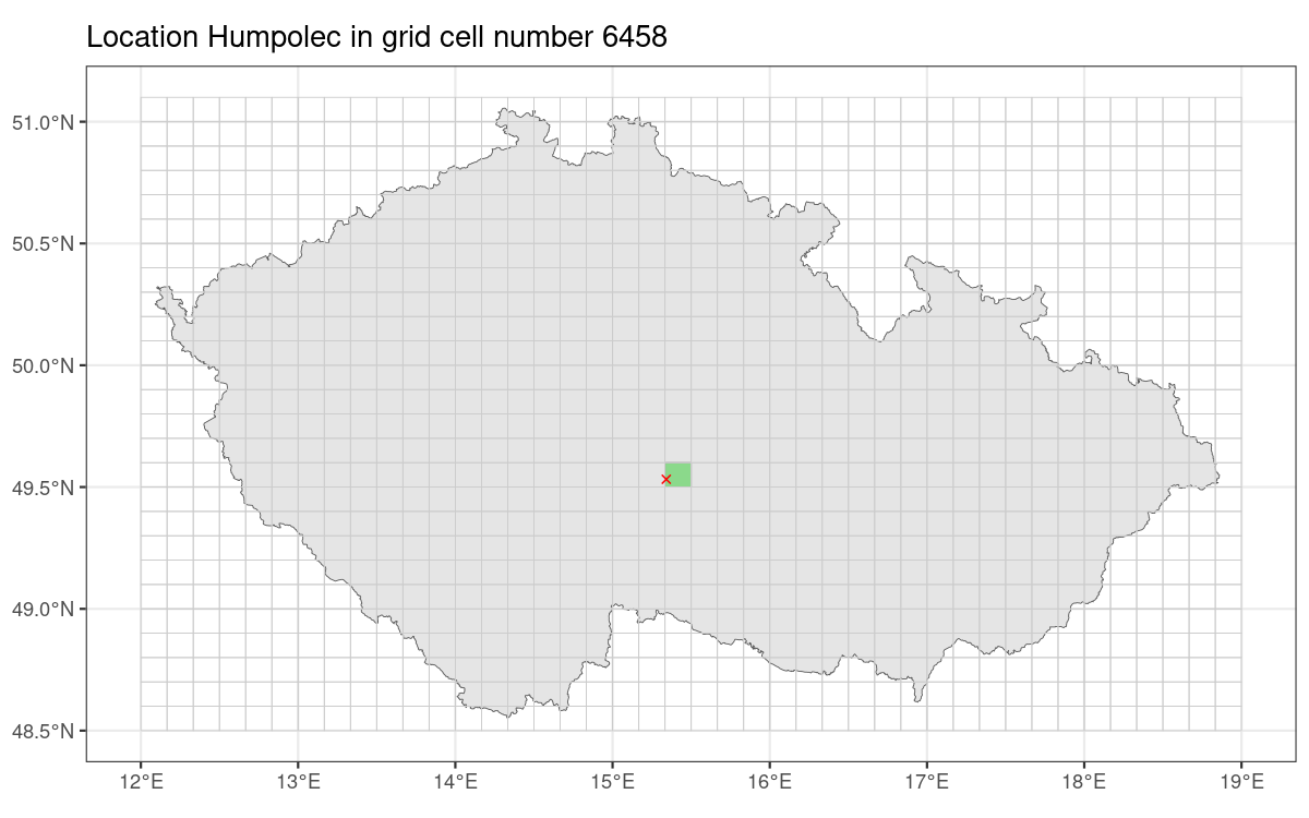
plot of chunk ctverce
Terrain of the Czech Republic
Understanding the lay of the land is important in many use cases in physical sciences; one of them is interpreting the flow of rivers.
Visualizing the slope & height of terrain is an important first step in understanding it.
Package RCzechia supports two versions of relief visualization:
- actual elevation model (meters above sea level)
- shaded relief
This example covers the first option.
library(RCzechia)
library(ggplot2)
library(terra)
library(tidyterra)
library(dplyr)

# terrain cropped to "Czechia proper"
relief <- vyskopis("rayshaded", cropped = TRUE)

# report results
ggplot() +
  tidyterra::geom_spatraster(data = relief) +
  scale_fill_gradientn(colors = hcl.colors(50, "Grays"), # 50 shades of Gray...
                       na.value = NA,
                       guide = "none") +
  geom_sf(data = subset(RCzechia::reky(), Major == T), # major rivers
          color = "steelblue", alpha = .5) +
  labs(title = "Czech Rivers & Their Basins",
       fill = "Altitude") +
  theme_bw() +
  theme(axis.title = element_blank(),
        legend.text.align = 1,
        legend.title.align = 0.5)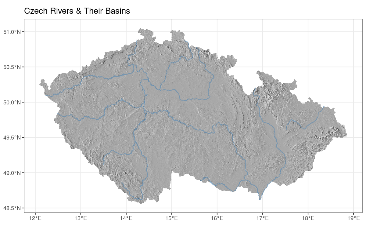
plot of chunk relief
Senate Elections of 2020
Visualizing election results is one of typical use cases of the RCzechia package.
This example uses {rvest} to scrape
the official table of results of the 2020 fall Senate elections from the
official site of the Czech Statistical Office, and display a map of the
party affiliation of the elected senator.
Since not all districts were up for election in this cycle two thirds of the map contain NA’s; that is expected behavior (the Czech senate elections are staggered, like in the US).
library(RCzechia)
library(ggplot2)
library(dplyr)
library(rvest)

# official result of elections from Czech Statistical Office
vysledky <- "https://www.volby.cz/pls/senat/se1111?xjazyk=CZ&xdatum=20201002&xv=7&xt=2" %>%
  xml2::read_html() %>%  # because rvest::html is deprecated
  html_nodes(xpath = "//*[@id=\"se1111_t1\"]") %>%  # get the table by its xpath
  html_table(fill = T) %>%
  .[[1]] %>%
  dplyr::select(OBVOD = Obvod, strana = `Volebnístrana`) %>%
  # pad OBVOD with zero to 2 places to align to RCzechia data format
  mutate(OBVOD = stringr::str_pad(OBVOD, 2, side = "left", pad = "0"))

podklad <- RCzechia::senat_obvody("low") %>%
  # match by key; left to preserve geometry of off cycle districts (NAs)
  left_join(vysledky, by = "OBVOD")

ggplot() +
  geom_sf(data = RCzechia::republika(), size = .85) + # Czech borders
  geom_sf(data = podklad, aes(fill = strana)) +
  labs(title = "Senate elections 2020") +
  theme_bw()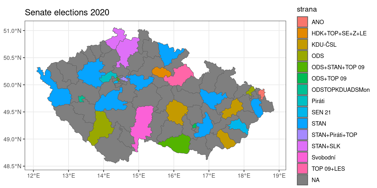
plot of chunk senat